How to Optimize Amazon Redshift for Faster and Seamless Data Migration

When it comes to handling massive datasets, choosing the right approach can make or break your system’s performance. In this blog, I’ll take you through the first half of my Proof of Concept (PoC) journey—preparing data in Amazon Redshift for migration to Google BigQuery. From setting up Redshift to crafting an efficient data ingestion pipeline, this was a hands-on experience that taught me a lot about Redshift’s power (and quirks). Let’s dive into the details, and I promise it won’t be boring!

Step 1: Connecting to the Mighty Redshift

Imagine having a tool capable of handling terabytes of data with lightning speed—welcome to Amazon Redshift! My first task was to set up a Redshift serverless instance and connect to it via psql.

Here’s how I cracked open the doors to Redshift:

psql -h <your-redshift-hostname> -p <port-number> -U <your-username> -d <your-database-name>

Once I was in, I felt like stepping into a data powerhouse. The next step? Building a table that’s smart, efficient, and ready for action.

[ Also Read Part 2: Automating Data Migration Using Apache Airflow: A Step-by-Step Guide ]

Step 2: Crafting a Supercharged Table

Tables are the backbone of any database, and in Redshift, designing them smartly can save you a world of pain. I created a users table with a structure optimized for Redshift’s columnar architecture and distribution capabilities:

CREATE TABLE users ( user_id INT PRIMARY KEY, first_name VARCHAR(50), last_name VARCHAR(50), email VARCHAR(100), created_at TIMESTAMP, last_login TIMESTAMP ) DISTSTYLE KEY
DISTKEY(user_id) SORTKEY(user_id) ENCODE BYTEDICT;

Here’s what makes this setup special: 

• DISTSTYLE KEY & DISTKEY (user_id):
  The DISTSTYLE KEY setting, combined with DISTKEY(user_id), is a clever way to ensure that the data is distributed evenly across all compute nodes. When you use DISTSTYLE KEY, Redshift distributes the data based on the specified column—in this case, user_id. This minimizes the data shuffling that can happen during query execution, which is especially important for large datasets. By choosing user_id as the distribution key, Redshift can better handle queries that filter or join on this column without needing to move data across nodes. 
• SORTKEY (user_id):
  Sorting the data by user_id helps Redshift quickly locate the records it needs when executing queries that filter by user_id. Think of it like arranging a set of books by author’s last name—if you know the author, you can jump straight to the right section. With the SORTKEY on user_id, Redshift doesn’t have to scan the entire table. It can skip irrelevant data, making retrieval faster. 
• Column Compression (ENCODE BYTEDICT):
  Redshift’s columnar storage and compression capabilities are key to making large datasets manageable. I used the BYTEDICT encoding to compress columns, which stores repeating values as a dictionary. This technique reduces storage space and speeds up query performance because fewer bytes need to be read from disk. It’s a space-saver that also enhances I/O efficiency.

[ Are you looking: AWS Database Migration Services] 

Step 3: Inserting Test Data—The Fun Begins! 

Why test with boring, clean data when you can simulate the real-world mess? I created 200 rows of diverse data with: 

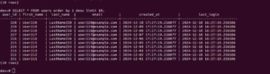
1. Skewed User IDs (150–160):
   Because real-world data isn’t always evenly distributed. This tested how well Redshift handles imbalances. 
2. NULL Values:
   Every 10th row had NULL values for created_at and last_login—because life is messy, and so is data. 
3. Randomized Timestamps:
   For added realism, I introduced randomized timestamps. Data should feel alive, right? 

Here’s the Python script I wrote to bring this to life: 

https://github.com/ramneek2109/DataMigration/blob/main/test_data.py 

 The result? A realistic dataset that was ready to be challenged! 

Step 4: Loading Data Like a Pro with the COPY Command 

When it comes to moving large datasets, Redshift’s COPY command is a game-changer. It’s fast, efficient, and designed for scale. For this PoC, I loaded a compressed CSV file stored in Amazon S3. 

But here’s the twist: 10 records in the file conflicted with existing user_id values in the users table. If I tried loading directly, it would fail. So, I got creative. 

Step 4.1: Load Data into a Staging Table 

First, I used a staging table to load all data safely without disrupting the existing table: 

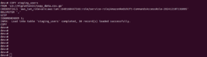
CREATE TEMP TABLE staging_users ( user_id INT, first_name VARCHAR(100), last_name VARCHAR(100), email VARCHAR(100), created_at TIMESTAMP, last_login TIMESTAMP ); COPY staging_users FROM 's3://<your-s3-bucket-path>/<file-name>.csv.gz' CREDENTIALS 'aws_iam_role=<your-iam-role>' DELIMITER ',' GZIP IGNOREHEADER 1; 

Step 4.2: Insert Non-Conflicting Records 

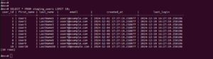
Next, I inserted only the non-conflicting rows into the users table: 

INSERT INTO users (user_id, first_name, last_name, email, created_at, last_login) SELECT s.* FROM staging_users s LEFT JOIN users u ON s.user_id = u.user_id WHERE u.user_id IS NULL; 

With this approach, I ensured that only unique user_id records made it into the users table. 

The rest? Skipped like a pro. 

Finally, I cleaned up the staging table: 

DROP TABLE staging_users; 

What I Learned (and Why It Matters) 

This part of the PoC taught me some valuable lessons: 

1. Optimization is Everything:
   Redshift’s performance relies heavily on how you design your tables. Choosing the right distribution and sort keys is key to unlocking its full potential. 
2. COPY Command is Your Best Friend:
   It’s fast, efficient, and handles large data like a champ. Pair it with staging tables for ultimate control. 
3. Test Like It’s Real:
   Simulating real-world scenarios with skewed data, NULL values, and conflicts helped me prepare for edge cases during the migration. 

 This was just the first step in my journey. In the next part of this blog series, I’ll delve into migrating this data from Redshift to BigQuery using the power of Apache Airflow. It only gets more exciting from here—stay tuned!